A primer on the Euler method for ODEs with Python

A recounting of my high school Python escapades, and the story of how I accidentally rediscovered the Euler method.

So, you want to solve an ordinary differential equation, but you want the computer to do it for you. Let’s look at a simple ODE.

\(\frac{dy}{dx}=-xy\)

Or, as some prefer it,

\(y'(x)=-xy(x)\)

Where y(x) is a differentiable function. Now, for the exact solution for some initial condition like y(0)=1, we find,

\(\ln|y|=\frac{-x^2}{2}+C\)

\(y=e^{\frac{-x^2}{2}+C} \rightarrow y=Ce^{\frac{-x^2}{2}}\)

\( 1=Ce^{\frac{0^2}{2}} \rightarrow 1=C\)

\(y=e^{\frac{-x^2}{2}}\)

That was quite friendly, but a computer did not do this, and that isn’t what we want. This solution will prove very useful, both for devising our solution, and for evaluating how it performs. Story time.

Long ago, during high school, I took a coding class in Python. Under circumstances I no longer recall, I ended up faced with the problem of simulating projectile motion, as many precocious teens are. More importantly to our story, however, I was frustrated by my failure to make it feel less floaty and more accurate and decided that I would give air resistance a shot. With nobody to tell me otherwise, I figured it couldn’t be that hard.

There was only one force acting on my projectile, gravity, which as we know can be abstracted as a constant acceleration given sufficient handwaving. To facilitate this, I expressed the projectile’s motion in the plane by its velocity. In the x direction, it was constant — the same as the launch velocity’s x component for the whole flight. For y, however, I would subtract gravity times the timestep to account for the acceleration of gravity toward the ground.

\(\frac{dx}{dt}=v_0\cos(\theta)\textrm{, } \frac{dy}{dt}=v_0\sin(\theta)-gt\)

Unknowingly, I was already solving a differential equation — the similarity of this to the solution for the full problem will become apparent soon. In fact, the y component’s exact solution is better known as one of the algebraic “kinematic equations” of classical mechanics,

\(d=v_0t+\frac{at^2}{2}\)

So, I knew if I wanted to implement air resistance, which acts in opposition to the direction of the motion, I would need to modify the equations, both referring to the next timestep’s velocity, to also include reference to the current velocity. I also added the coefficient of drag so I could tune the resistance to what was accurate or what felt the best¹.

\(\textrm{Let } F_D=\frac{1}{2}\rho v^2C_DA\)

\(a_D(v)=-\frac{\rho v^2 C_D A}{2m}\)

\(\frac{dx}{dt}=v_0\cos(\theta_0)+a_D(v)\cos(\theta)t \textrm{, } \frac{dy}{dt}=v_0\sin(\theta_0)-gt+a_D(v)\sin(\theta)t\)

\(\theta=\tan \left( \frac{v_y}{v_x} \right)\)

Which expands to,

\(x_t=x_0+\int^t_0 v_0\cos(\theta_0)+a_D(v)\cos(\theta)t\,dt\)

\(y_t=y_0+\int^t_0 v_0\sin(\theta_0)-gt+a_D(v)\sin(\theta)t\,dt\)

Thus, I had a way to determine the velocity at the next timestep using the velocity at the current timestep, including air resistance. At the end of each timestep, I would then add the derivatives to the current position and pass them off to the next timestep. Without understanding what I had done, and without formal instruction in calculus at the time, I had accidentally written a primitive ODE solver. More generally, this method is known as the forward (or explicit) Euler method and is expressed for first-order ODEs as:

\(y_{t+1}=y_t+hf(t, y_t)\)

Where f is our differential equation under examination. The validity of this method for solving any ODE falls out of the fundamental theorem of calculus in a very pleasing way. As the first theorem states that the integral of the derivative will yield the function, it would be similarly valid to say that many small summations of the small differences of a function accumulated over the domain will discretely approximate the function.

Indeed, this method is what I had been doing with the acceleration for gravity in the first place — adding the acceleration times some timestep to the current velocity to calculate the velocity at the next time step. I determined this logically, but the units also check out, as the timestep in seconds multiplied by the acceleration in meters per second squared will work out to be meters per second overall. This kind of check for units is very handy in many cases, this being just one example.

Regardless, let us discretize our prior problem so we can more easily express it in code. This is more faithful to how I came about this in the first place, too.

\(v_{x, t+h}=v_t\cos(\theta)+a_D(v)\cos(\theta)h\)

\(v_{y, t+h}=v_t\sin(\theta)-gh+a_D(v)\sin(\theta)h\)

Where h is the timestep of the simulation. So, let’s write it. We should start with our initial conditions. (The full code is available here for copy-pasting, or whatever)

Now, real quick, let’s add the star of the show.

Short and sweet, isn’t it? Here’s the less short and less sweet part, where all the annoying footwork to use this is. We end up solving a system of differential equations to satisfy our needs here since the x and y velocities end up relying on each other’s value due to their mutual dependence on the speed — that is, the magnitude of the velocity vector.

Cool. Now, when we call solve(), it will use the initial conditions I (embarrassingly) globally defined in the beginning, and:

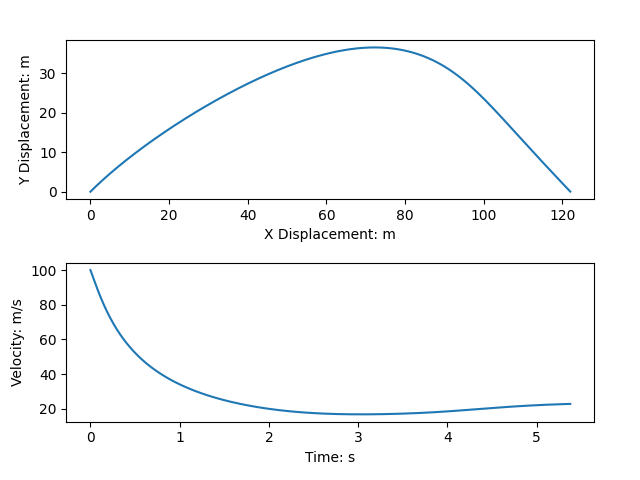
Would you look at that? A convincing and accurate trajectory determined by solving the system of differential equations that we set up. We have finally caught up to where I left off in high school, satisfied with the motion of this projectile.

Now, note that I chose a particularly small timestep for this at h=0.001. What happens if I raise it, decreasing the overall number of steps?

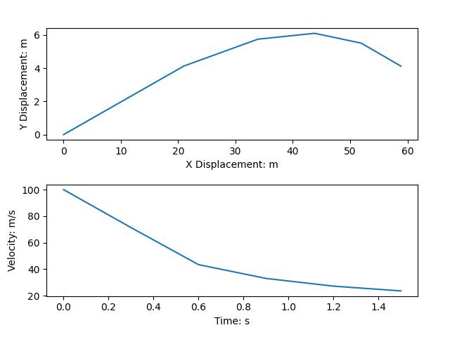
Well, that’s just wrong. For one, the Y displacement only goes up to… six? Compared to the over 30 it had achieved in the finer simulation, that’s a real problem. For this coarse simulation, I used h=0.3. Anything coarser, and the simulation will immediately phase into the earth – which we know to be false.

On some other problems, instead of giving an embarrassingly wrong answer, it will instead spin out of control due to what is known in the field of numerical methods (the field we are discussing) as numerical instability. Some problems, when faced with a step size that is too high, will oscillate violently and/or fly off to an extreme until your computer calls it a day.

Given all this, though, we still don’t know whether this even resembles what it is supposed to. After all, without an exact form, this could be completely wrong! But, to assuage this, let’s consider the first ODE – the one we also solved for the exact form. We can use the same method in a much simpler setup to solve this problem – proving not only that this generalizes, but also allowing us to examine the accuracy of each step size.

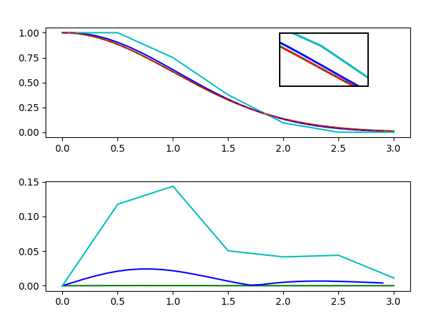
In dashed red in the top plot is the exact solution, with the green being h=0.001, the blue being h=0.1, and the cyan being h=0.5. Note that the green and blue are quite similar – the green being nearly indistinguishable from the exact solution in the detail view.

The second plot compares the error between the exact and estimated solutions over the simulation span, with there being a positive relationship between step size and error. This is not terribly rigorous, and further analysis is possible to formalize the error both in each step and accumulated across a simulation, but that is outside of scope.

1. Yes, I know it is a lot more complicated than this. Thankfully for all of us, I don’t care.