
A primer on the finite difference method (with Python)
An approachable view into solving PDEs
Introduction
A differential equation, broadly speaking, is a specific breed of equation that relates a function to its own derivative in some way. For example, in my prior post about the Euler method, the following example was given:
Or, in a more pertinent form to our following discussion:
Observe that the derivative of the function is defined by itself. This makes an exact solution non-obvious. Furthermore, note that only the first derivative is used, meaning this is a first-order differential equation. Finally, the function f is only of one variable, making this an ordinary differential equation. This discussion focuses on their older sister, the partial differential equation, which is of multiple variables.
As an aside, a function of multiple variables is very similar to a function of a single variable. The function we are familiar with takes in some value x and is equal to some value y for that x. A multivariable function takes in multiple values x and y and is equal to some value z for that combination of x and y. The multivariable function is not limited to two inputs, but for our discussion, it will be limited to two or three dimensions, correlated to spatial dimensions.
Let us now consider a simple partial differential equation and one that will be the subject of this post, Laplace’s equation:
Or, expanded to a form that may be more familiar, in two dimensions:
The partial derivative, denoted with the curly d, is a multivariate corollary of the derivative from introductory calculus. It simply expresses the same derivative as we know and love, but with all variables that are not being differentiated with respect to being treated as constants. As an example:
Laplace’s equation, from before, is a second-order partial differential equation, due to it being the second partial derivative.
Maxwell’s Equations
Maxwell’s equations are a set of partial differential equations that describe electromagnetism. They are arguably some of the most important equations ever to be penned to paper. Of interest to us today is the first equation, also known as Gauss’s Law, describing the electric field arising from charged particles:
Where rho is the charge density, and epsilon-naught is the permittivity of free space. We don’t need to be concerned with the meaning of those, as in our consideration of the problem, we will say that no free charges are floating around1, which will reduce the equation to:
The definition of the electric field, E, comes from the force that would be experienced by an example charged particle within the field, also known as a test charge. Furthermore, there is an associated potential energy, as the electric field is conservative, which is called electric potential. It follows that, much like gravity, the force associated with it will point towards lower potential energy. Or, put elegantly:
All together now:
We have now successfully shown that Gauss’s law combined with the definition of electric potential, when there is no charge density, is equivalent to Laplace’s equation. Regrettably, it is not nearly as simple to solve partial differential equations by hand as it is for ordinary differential equations.
An Adventure in Finite Differences
We’d like to solve this partial differential equation we derived, but as mentioned before, it is impossible to do so analytically. However, we have the power to make this hard problem into a simpler one by using approximations to get an answer that is close enough.
Let us begin with the definition of the derivative:
How can we find this without needing to take the limit? Let’s Taylor expand f(x+h):
And re-arrange:
On the left, there again is the definition of the derivative, but there are a lot of other things happening on the right. We can truncate these at the cost of accuracy, noting that the 1st power of h will have the largest impact on the error, permitting us to state:
Where big O is a way of expressing how fast the error goes to zero as h approaches zero — in this case, it does so linearly. This is called the first-degree two-point forward finite difference. Let us now try f(x-h):
Interesting. We can also construct a finite difference from this, known as the first-degree two-point backward finite difference:
Now, what if we could combine the two? Let’s subtract the forward Taylor expansion from the backward:
Miraculously, we have yielded a second-order two-point central finite difference! Observe that the error is better here — the error now declines quadratically. Now, let’s solve for the second derivative. Let’s try adding the forward and backward finite differences, instead:
Perfect! Now, we have to apply this to multiple dimensions, such that we can solve our problem from before. Let’s change f to a function of multiple variables on a grid of equal spacing h, such that:
This is frequently referred to as the five-point stencil. We can further tailor this to Laplace’s equation by setting the left hand equal to zero. We can also set h to one, as we are now operating on a grid, and we presume that h is a single grid square.
And with that, we can now determine any given point in a 2D solution to Laplace’s equation. This happens to end up being the average of the points in cardinal directions from the point in question. Remarkably, this same expression that we have derived in the context of electric potential also applies to gravitational fields and is strongly related to the way heat diffuses through a region.
Boundary Conditions
This whole talk of grids has a concerning implication. Suppose we examine the region from (0,0) to (2, 2), indexing from zero. At (1,1), our finite difference will behave fine, having points on all sides to reference, but the moment that it is in any other position, it simply will not work, as the region is outside of our domain. There are a few different approaches to handle this, but we will employ the one known as ghost points. The idea is that we can pad the boundaries of our solution with fictitious points, such that the finite difference will be able to get a value.
                                                                      ■■■■■
                                                                      ■□□□■
                                                                      ■□□□■
                                                                      ■□□□■
                                                                      ■■■■■
Where ■ are ghost points, and □ are part of the region.
The infinitesimal space between the hollow and filled squares, the boundary of the PDE region, is critical to the solution of the PDE. We must rigorously define these to get the behavior we want — as any solution to the PDE must also fulfill these boundary conditions to be correct.
First, let us examine the Dirichlet boundary condition. It simply states that at the boundary, the value is given by some (scalar) function, whether a constant or something else that is defined across the boundary. For us, that means the ghost points would have that value.
This permits the central difference to behave normally as if there were immutable points of this bordering the region. For example, in the consideration of electric potential, a grounded box would be represented as a Dirichlet with a value of 0, or for heat, a surface of constant temperature.
Next, the Neumann boundary condition instead defines the derivative of the boundary. For instance, we could define the derivative to be zero, which approximates infinite space2, or a perfect insulator for heat equations.
However, this does not answer the question of what the ghost points should be. Let’s consider solely the case where we’d like the derivative to be zero. It follows by the theorem of thinking about it really hard that the ghost point ought to equal whatever edge point we are considering the derivative from. We need not make the computer do this when we can just algebra it out. Recall that, for a center point:
Suppose we are at an upper edge boundary, such that y+h is out of bounds. We can substitute f(x, y) for that point, per our prior discussion, and solve:
Or, for the top right corner:
These all happen to end up being the average of the non-boundary surrounding points. We need not write all of these out, because of how we are going to end up solving this.
Convolution
Convolve is an unusual operator that can do some really neat things. The operator’s exact definition is a bit burdensome for how we are going to use it, so a description of its function will suffice. In our view, convolution occurs between an input matrix and a kernel (another matrix, generally smaller), and does the following:
Where omega is the kernel, with its center at 0. To convolve the image, for each point of the image, overlay the kernel’s center at each point, multiply the value of the kernel at each index with the image value “below” it, and sum all of that together. Consult the GIF:

Now, in retrospect to what we discussed regarding finite differences, it may quickly become apparent that these are related! If we use the kernel:
When convolved with the initial conditions we give the PDE, will satisfy Laplace’s equation. Note now that per our prior discussion, this will only work for points that don’t touch a boundary. To solve this, the key becomes that convolution is a linear operation. That is, if we multiply all values of the kernel by something, it will scale correctly as if we had done that in the first place. So, we can instead correct for this edge factor with another matrix of the same shape as g, which when taking the Hadamard (element-wise) product with the convolved image g, will correct these errors.
We need not modify the kernel itself for each edge, since the Neumann ghost points shall be of zero value and thus not contribute to the convolution value. Instead, this adjusts the scaling of the points we care about to align with the formal definitions, that is, to re-create the “average” of the surrounding points.
The other thing that may be apparent is that only one pass will be woefully inadequate.
Instead, we must repeatedly do this until the answer stops changing significantly, a state known as convergence, for a method known as relaxation. The other thing is that this operation deleted our “electrode” of 1V in the center — which happens to be a Dirichlet condition. We will need to re-set these each time.
Making the computer do it
It happens to be that computers, and specifically GPUs, are good at this whole convolution thing, seeing as it is important to convolutional neural networks. As such, this will be built around PyTorch, which is arguably the greatest GPU acceleration framework ever created. If you do not have a GPU, PyTorch runs the operations flawlessly on the CPU faster than Numpy can. Let’s take what we have discussed and turn it into code:
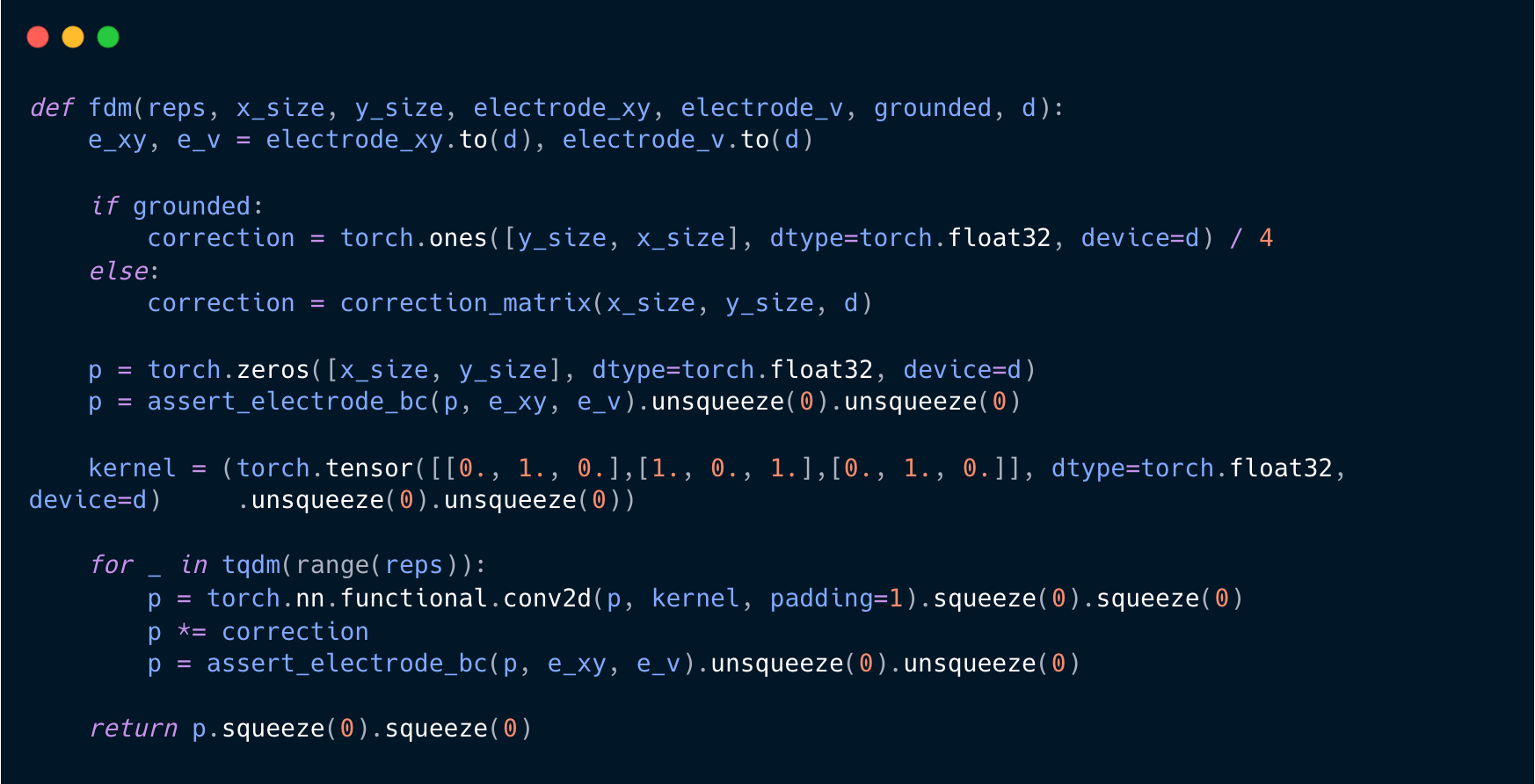
That’s all! That is the code that produces the finite difference method. First, it generates the correction matrix, checking for whether we would like the edges to be grounded, correlating to Dirichlet boundary conditions. Otherwise, it generates the correction matrix from before. Next, it creates the potential field upon which it operates, asserts the electrodes as our initial condition, and defines the generic kernel3. Next, for however many repetitions we tell it to go, it convolves the kernel with the potential field — padding it with zeros around the edge. Next, it applies the correction and reasserts the electrodes. The rest of the code is largely uninteresting and supporting to this main part, but will be available at the bottom.

Here, at the 1/3rd mark, an electrode at 1V is placed across the field. Then, at the 2/3rds mark, an electrode at 0 volts. Note how between the electrodes, there is a linear relationship between voltage and distance — in line with the analytical model of the same situation. We can try something more complicated, instead.

This is an example of an Einzel lens, which is a type of lens for charged particles.
Next Steps
That is the conclusion of the scope of this post. There are a few things that have been left out so far. Firstly, one could exploit the linearity of Laplace’s equation to be able to efficiently compute changes in electrode voltage, say, for radio-frequency electrodes. Another thing, and probably of very high priority, is to improve how many repetitions the model takes. A usual approach is to set a threshold of convergence that is compared to the sum of the absolute value of all changes to the potential field — if it is at or below that, the field has converged, but otherwise, it can run another batch.
The elephant in the room is to utilize this to simulate the flight of ions through this space. This is, at first sight, a simple task — but becomes hairier as one realizes that most ions are very light, and as such get moving alarmingly fast quite quickly, eventually requiring relativistic correction. Furthermore, if you have a beam of charged particles, they will mutually repel each other, amongst other nasty surprises.
All of this quickly becomes a headache.
Further Reading
Introduction to Electrodynamics, David Griffiths
A formidable introduction to the subject, some of the discussion here was informed by chapters 2 and 3.
Simulating Fields, Ions, and Optics, Ian Anthony
Being the inspiration for this post, it takes a much less formal approach, substituting for much stronger visuals. Try out the playground, it is very neat!
Surprisingly cordially written, this abridged manual has some valuable tidbits about the theoretical and practical underpinnings of the problem discussed.
We can get away with this by saying that the voltages are introduced by external charge distributions, like from within a battery.
This is a tricky problem, unfortunately, but generally, it doesn’t disturb the things you want to investigate, which are usually ion lenses where all interesting results are contained within the lens. SIMION has an extensive and very clear discussion.
It must be unsqueezed because torch.nn.functional.conv2d requires two extra dimensions out front.